Geometric Brownian Motion

Geometric Brownian motion (GBM) is a type of random walk model that produces movements reminiscent of stock price charts. Its data generating process (DGP) describes exponential growth perturbed by normally distributed random shocks.

The value of a GBM process S_t changes as defined in the following stochastic differential equation (SDE):

\begin{align}
dS_t = r S_t dt + \sigma S_t dW_t
\end{align}

\begin{aligned}
S_t &: \mathrm{value~at~time}~t\\
r &: \mathrm{growth~rate}\\
\sigma &: \mathrm{volatility}\\
W_t &: \mathrm{Wiener~process}
\end{aligned}

In Equation (1) the deterministic term rS_tdt drives exponential growth and the stochastic term σS_t​dW_t​ contributes random shocks. Within the stochastic term, it is the Wiener Process^[4] W_t that causes the random variability. Wiener Processes integrate Gaussian white noise and have the following basic properties:

\begin{align}
&W_0 = 0\\
&W_{t}  \sim~N(0,t)
\end{align}

As an additional characteristic of white noise non-overlapping increments of W_t are independent.

The SDE in (1) integrates to the following analytical solution in Itô calculus^[1]:

\begin{align}
S_t = S_0~e^{(r - \frac{\sigma^2}{2})t + \sigma W_t}
\end{align}

Intuitively, since E[W_t] is zero, the expected value of S_t is still geometric growth unperturbed by random shocks:

\begin{aligned}
E[S_t] = S_0 ~ e^{rt}
\end{aligned}

GBM in discrete time-steps

Simulations and other practical applications of GBM use a discrete time-step version of Equation (1). Because of their distribution given in (3), increments dW_t over timespan Δt have a variance of Δt. Therefore, the aggregate increment ΔW_t can be expressed as:

\begin{aligned}
\Delta W_t = \sqrt{\Delta t} ~ \epsilon_t\\
\epsilon_t \overset{\mathrm{iid}}{\sim} N(0,1)
\end{aligned}

Consequently, the discrete version of Equation (1) is given by:

\begin{align}
\Delta S_t &= r S_t \Delta t + \sigma S_t \sqrt{\Delta t} ~\epsilon_t
\end{align}

In computational statistics, the independently and identically distributed (iid) shocks ϵ_t are simply draws from a standard normal distribution. It is thus straightforward to obtain GBM paths starting from some initial value S_t and recursive applications of Equation (5).

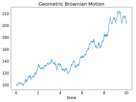
Figure 1 shows an example of a geometric Brownian trajectory starting at 100 with 4% annual growth and 10% volatility developed over a 10-year period. Because of the similarity of geometric Brownian motion to stock market prices, economists sometimes use projections from such random paths to price derivatives.

Mathematical Derivation of GBM Returns Using Itô Calculus

To get the investment return, we rewrite the GBM process from Equation (1) in terms of logarithms. Doing so requires Itô calculus^[1] approximating infinitesimals as second order Taylor series expansions:

d(f(x)) = \frac{\partial{f(x)}}{\partial{x}}dx + \frac{\partial^2{f(x)}}{2~\partial{x}}dx^2

Plugging in f(x)=ln(x):

\begin{aligned}
\frac{\partial ln(S_t)}{\partial S_t} &= \frac{1}{S_t}\\
d(ln(S_t)) &= \frac{dS_t}{S_t} - \frac{1}{2}\frac{dS_t^2}{S_t^2}\\
\end{aligned}

The term dS_t² is the quadratic of the SDE given in equation (1):

\begin{aligned}
dS_t^2 = &~dS_t \cdot dS_t\\
dS_t^2 = &~r^2 S_t^2 dt^2\\
&+ 2~r\sigma~dt~dW_t\\
&+ \sigma^2 S_t^2 dW_t^2
\end{aligned}

In calculus, as dt→0, dt² approaches zero more quickly. Similarly for the product dt⋅dW_t. However, dW_t² is proportional in expectation to dt because the variance of W_t is t. So dW_t² is the only term that impacts the result for dS_t², contributing a deterministic drift of O(t). Substituting in the Taylor series expansion:

\begin{aligned}
d(ln(S_t)) &= \frac{dS_t}{S_t} - \frac{1}{2}\frac{dS_t^2}{S_t^2}\\
d~lnS_t &= \frac{dS_t}{S_t} - \frac{1}{2}\sigma^2dt
\end{aligned}

The logarithmic variant of the GBM process equation is then given as:

\begin{align}
d~lnS_t &= (r - \frac{\sigma^2}{2})dt + \sigma dW_t
\end{align}

This proves that, when looking at returns, the expected growth r of GBM paths is diminished by a volatility term σ²/2. Since E[σdW_t] is zero, the expected return μ follows as:

\begin{align}
\mu = r - \frac{\sigma^2}{2}
\end{align}

Furthermore, solving SDE (1) is now straightforward by first integrating differential equation (6) over time:

\begin{aligned}
ln(S_t) &= \int (r - \frac{\sigma^2}{2})dt + \sigma dW_t\\
ln (S_t) &= (r - \frac{\sigma^2}{2})t + \sigma W_t
\end{aligned}

Equation (4), the solution to SDE (1), is now obtained by applying the exponential function and setting a start condition of S_t(0)=S₀.

Derivation of GBM-Variance

Finally, a short derivation of the variance of GBM paths. Generally, the variance of a random variable follows from its first and second moments:

\begin{align}
Var[X]  &=E[X^2] - E[X]^2
\end{align}

From equations (6) and (7) follows that the instantaneous return GBM paths is normally distributed with mean μ and variance σ²:

\begin{align}
d~ln(S_t) &\sim N(\mu, \sigma^2)
\end{align}

Per definition a random variable is lognormally distributed when its logarithm is normally distributed. Now define a lognormally distributed random variable X as:

X = e^{d~ln(S_t)}

The moments E[X] and E[X²] can be taken from the moment generating function for lognormal variables^[3]:

E[X^n] = exp(n\mu + \frac{n^2\sigma^2}{2})

The first and second moments are therefor given as:

\begin{align}
E[X] &= e^{\mu + \frac{\sigma^2}{2}}\\
E[X^2] &= e^{2 \mu + 2 \sigma^2}
\end{align}

Plugging equations (10) and (11) into (8) yields:

\begin{align}
Var[X] = e^{2\mu + \sigma^2}(e^{\sigma^2}-1)
\end{align}

In line with the definition of moment generating functions^[2] the result from equation (12) is valid for a lognormally distributed random variable having a unit value of one at time zero. For a GBM path starting with a value S₀ at time zero, which is integrating up the infinitesimals from equation (9), the moments will be:

\begin{aligned}
E[S_t] &= S_0~e^{(\mu + \frac{\sigma^2}{2})~t}\\
E[S_t^2] &= S_0^2~e^{(2 \mu + 2 \sigma^2)~t}
\end{aligned}

Substituting back r = μ + σ²/2, we get the expected value and variance of GBM paths:

\begin{aligned}
E[S_t]&=S_0e^{r t}\\
Var[S_t]&=S_0^2e^{2r t}(e^{\sigma^2 t} -1)
\end{aligned}

References

[1] Itô calculus: Wikipedia.org

[2] Moment Generating Functions: Statlect.com

[3] Moments of Lognormal Distribution: Statlect.com

[4] Wiener Process: Wikipedia.org

Related Publications

Geometric Brownian Motion in German: zinseszins.de