Monte Carlo simulation is a simple means of estimating returns on complex financial instruments. This is demonstrated using the example of the expectation, rate of return and variance of geometric Brownian motion (GBM).
Because of its similarity to financial time series, GBM is a basis for popular derivatives pricing models, such as the Black Scholes formula for options. A key characteristic of GBM is that its expected return differs from its deterministic growth rate. However, gaining a mathematical understanding of these lognormal properties requires stochastic calculus. Instead of mastering complex mathematics, Monte Carlo simulation offers itself as a simple alternative to estimate values in an empirical manner that works even when no analytical models exist.
Since a large number of identically distributed independent (iid) samples is needed for Monte Carlo simulation, the article starts off with a computational algorithm for generating GBM paths. Next Monte Carlo simulation formulas are introduced, which essentially average over iid samples. Finally, the results from a computational experiment are compared to what the mathematical GBM model predicts in theory.
Discrete Time-Step GBM
Monte Carlo samples for geometric Brownian motion can be obtained from recursive applications of the discrete time-step variant of the GBM differential equation:
\begin{align}
\Delta S_t &= r S_t \Delta t + \sigma S_t \sqrt{\Delta t} ~\epsilon_t
\end{align}
\begin{aligned}
S_t &: \mathrm{value~at~time}~t\\
r &: \mathrm{growth~rate}\\
\sigma &: \mathrm{volatility}\\
\Delta t &: \mathrm{discrete~time~step}\\
\epsilon_t &\overset{\mathrm{iid}}{\sim} N(0,1)
\end{aligned}First, the simulation algorithm must choose a small but essentially arbitrary time span Δt, an initial value S0 at time zero, and draw independent, normally distributed (iid) shocks ϵt from a random number generator. GBM paths are then obtained by accumulating a large number of ΔSt as stated in equation (2):
\begin{align}S_{t+1} = S_{t} + \Delta S_t
\end{align}
What the simulation will be aiming to verify is that the expected return R indeed differs from the growth rate r. Furthermore, it will estimate the GBM variance. In theory, these values should be as follows:
\begin{aligned}
E[S_t] &= S_0~e^{rt}\\
E[R] &= r - \frac{\sigma^2}{2}\\
Var[S_t] &= S_0^2~e^{2rt}(e^{\sigma^2t}-1)
\end{aligned}Monte Carlo Simulation Experiment and Formulas
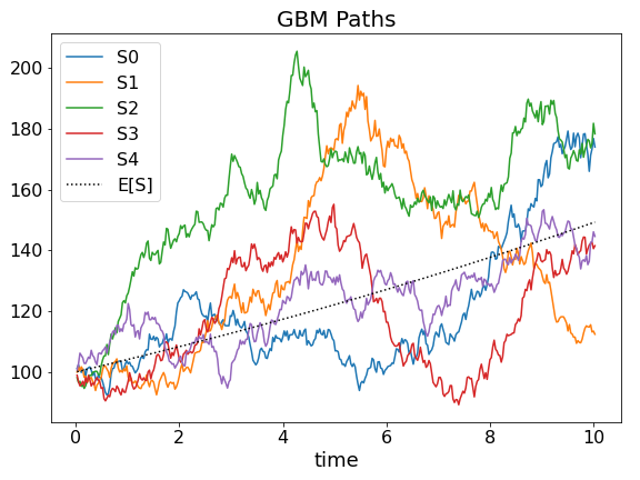
The properties of GBM will now be estimated in an experiment with 10,000 Monte Carlo paths. Figure 1 shows five such sample GBM paths averaging around the expected path value as a dotted line. Simulation parameters for equation (1) are r=4%, σ=10%, Δt=7 days, and S0=100 as a start value for the recursion. Furthermore, the simulation time span is 10 years giving a total of 522 data points per path. GBM properties can now be estimated using the following general set of Monte Carlo formulas:
\begin{align}
\bar{S_t} &= \frac{1}{N}\sum_{i=0}^{N}{S_{ti}}\\
Var[S_t] &= \frac{\sum_{i=0}^{N}{(S_{ti}-\bar{S_t})^2}}{N-1}\\
Var[\bar{S_t}] &= \frac{1}{N}Var[S_t]\\
R_{ti} &= \frac{1}{t}log(\frac{S_{ti}}{S_0})\\
\bar{R_t} &= \frac{1}{N}\sum_{i=0}^{N}{R_{ti}}\\
Var[R_t] &= \frac{\sum_{i=0}^{N}{(R_{ti}-\bar{R_t})^2}}{N-1}\\
Var[\bar{R_t}] &= \frac{1}{N}Var[R_t]\\
\end{align}
\begin{alignat*}{2}
\bar{S_t} &&~:~ &\mathrm{mean ~ path ~ value}\\
R_{ti}&& ~:~ &\mathrm{investment ~ return}\\
&&&\mathrm{for~path}~i\\
\bar{R_t} &&~:~&\mathrm{mean~investment}\\
&&&\mathrm{return}\\
i &&~:~&\mathrm{scenario~index}\\
\end{alignat*}In equations (5) and (9) variances of the mean are lower than overall variances as a consequence of the Central Limit Theorem[1]. This gain in precision is of course the whole point of running Monte Carlo simulations with a high number of scenarios. The mean values from Equations (3) and (7) then serve as consistent estimators for the expected values of paths and investment return.
\begin{align}
\widehat{E[S_t]} &= \bar{S_t}\\
\widehat{E[R_t]} &= \bar{R_t}
\end{align}
Just the deterministic growth rate isn’t directly observed in the Monte Carlo simulation. It can, however, be obtained by rewriting the equation for E[St] in terms of the growth rate r:
\begin{aligned}
\widehat{E[S_t]} &= S_0~e^{\hat{r} t}\\
\Leftrightarrow\hat{r} &=\frac{1}{t}ln(\frac{\widehat{E[S_t]}}{S_0})
\end{aligned}Results for Monte Carlo Simulation of Returns
The Monte Carlo simulation produces the following estimates for the GBM paths of the experiment:
| Property | Estimate | 95% CI |
|---|---|---|
| E[St] | 149.33 | 148.38 – 150.29 |
| r | 4.0082% | 3.9442 – 4.0719% |
| Var[St] | 2368.7 | N/A |
| E[Rt] | 3.5037% | 3.4414 – 3.5659% |
The estimate of the growth rate r calculated from E[St] is close to the initial and theoretical value of 4% and the expected return on investment E[Rt] runs about 0.5% below the growth rate. With a value of σ = 10% corresponding to σ2/2 = 0.5%, this difference between deterministic growth and expected return is very close to what theory predicts. A seemingly contradictory yet very important and useful advice for all kinds of investment strategies: volatility is bad for returns!
Finally, plugging r=4%, S0=100, σ=10% and t=10 into the formula for Var[St] gives a theoretical variance of 2340.62. That’s also not too far off the estimate of 2368.7. Monte Carlo simulation does work!
References
[1] Central Limit Theorem: Wikipedia.org