Optimize Portfolios Calculating Logarithmic Returns

Calculating logarithmic returns is a simple risk and volatility pricing method allowing retail investors to optimize investment portfolios. The proposed technique determines the proportion of a risky position in an overall portfolio that maximizes investment performance. Accordingly, a reduction of the size of leveraged positions can swing portfolio returns from the negative into the positive. Moreover, by taking a logarithmic view of the impact of price declines, risk management becomes an integral part of the trading strategy.

The introduction explains why most investors suffer losses with highly volatile positions such as CFDs or futures, even when price forecasts are largely correct. A simple procedure is then described for optimally weighting risky positions in the overall portfolio. The article concludes with mathematical derivations, an understanding of which is not essential to the application of the optimization method.

Why do Most Retail Investors Make Losses with CFDs and Futures?

Contracts for Differences (CFDs)^[2] and futures are investment instruments whose value derives from the difference between entry and exit prices. Depending on leverage, strong profits or losses may result which, calculated in absolute percentages, tend to cancel each other out. For instance, a transaction with 90% profit followed by one with a 90% loss may sound like a zero-sum game. However, a loss of just 52.6% is enough to undo a 90% gain. A 90% loss, on the other hand, requires a gain of 900% to compensate! Unfortunately, the problem only becomes apparent in repeated transactions.

A Practical Example with 70% Accuracy of Predictions

Suppose it were possible to predict rising or falling prices in the financial markets with 70% accuracy. Chart technicians will concede that this is not easy to achieve even for professionals. In fact, financial time series often resemble random paths that could well be geometric Brownian motion^[3], making the contrarian view of unpredictable short term fluctuations in stock prices popular among economists.

As a second assumption for the example, a leveraged investment instrument is expected to either increase 90% in value when market prices rise, or decrease by 90% when prices fall.

The expected value of this bet, which is equivalent to the average investment success, is straightforward to determine. According to probability theory, it is calculated from the two possible outcomes weighted by their respective probabilities. If in 70% of cases a stake rises from $100 to $190, and in 30% of cases it falls to $10, then its expected or mean value is 0.7 times $190 plus 0.3 times $10, equaling $136:

Average = 70% * 190 + 30% * 10
        = 133       + 3
        = 136
Gain    = (136 - 100) / 100 = 36%

So, in line with the computed average, the model investment should pay a 36% gain. However, calculating averages of absolute gains and losses ignores reinvestment effects and is therefore misleading. Figure 1 illustrates this problem. The sad reality is that 65.7% of investors lose money if they repeat the trade three times. Despite a fabulous hit rate of 70% of price predictions!

Portfolio Value Scenarios in a Binomial Tree

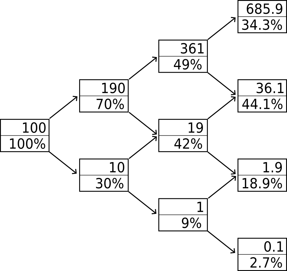
Possible valuations of a risky portfolio that shall be optimized calculating logarithmic returns in a binomial tree. — Figure 1: Evolution of portfolio values in three iterations of an investment with a ±90% gain and a 30% probability of loss. Nodes show portfolio values in their upper halves and probabilities in % in their lower halves.

Figure 1 shows a so-called binomial tree^[1] of the possible outcomes of repeating a transaction as described in the previous section three times, with a stake of $100, a profit of ±90% and a success rate of 70%. Each node represents a scenario and arrows indicate portfolio values moving up or down. Nodes have portfolio values in their upper halves and probabilities of being reached in their lower halves.

On the far left, at the root of the tree, is the initial portfolio value of $100 available with certainty, that is, a probability of 100%. The first step consists of the two outcomes already discussed, $190 and $10. In the second step there are three possible outcomes of €361, €19 and €1. Finally, the third step produces the four possible end results on the far right of the tree. These amount to $685.9, $36.1 and the practical total losses of $1.9 and $0.1. Investors only make profits at the top-right node. Since it is only reached in 34.3% of cases, this means that the overall probability of losses amounts to the already mentioned 65.7%, which can be computed by adding up the individual probabilities of the three lower nodes on the right hand side:

Prob. of loss = 44.1% + 18.9% + 2.7%
              = 65.7%

The many losers face 34.3% of winners pocketing fabulous gains of 585.9%. The reality of CFD investing appears to be even worse if official warnings of more than 80% of retail accounts performing unfavorably hold true. After all, hardly any investor can predict financial rates with an accuracy of 70%.

A detailed discussion of the mathematics of binomial trees is out of scope here. Instead, interested readers are encouraged to study the provided Excel sheet.

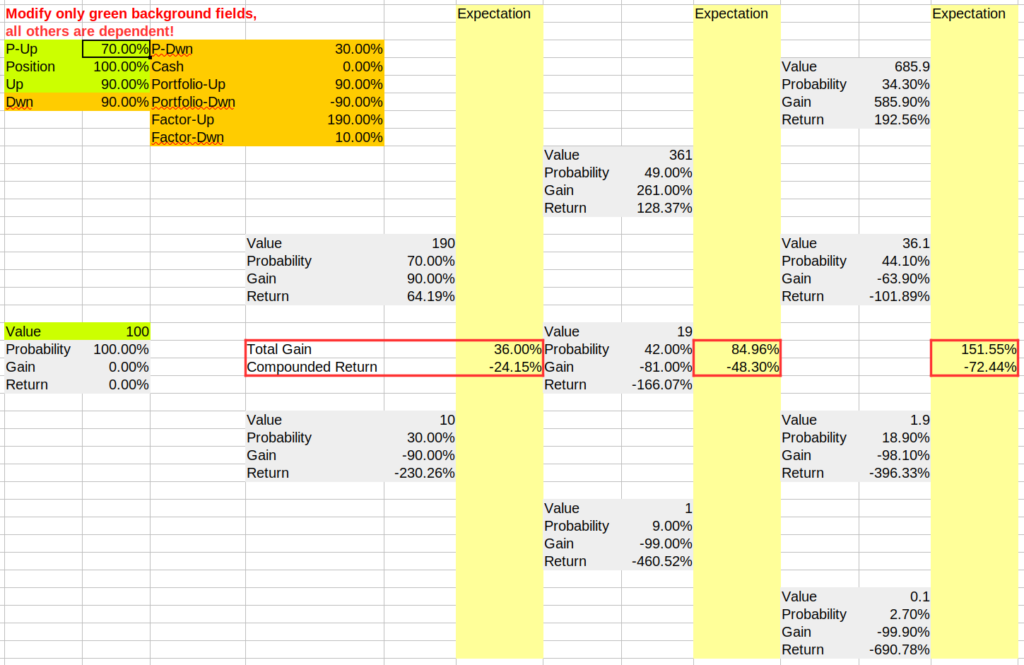
Screenshot of an Exel-Sheet for the optimization of portfolios holding highly risky positions. — Figure 2: Screenshot of the portfolio analysis in Excel. Cells with red frames contain logarithmic returns alongside absolute gains.

The Excel sheet opens by clicking this link.

Correctly Calculate Returns on Risky Positions

Summing up the previous sections, the portfolio discussed brings losses for most investors, although individual transactions promise average gains of 36%. Clearly, an absolute transaction profit does not guarantee long term success as reinvestment effects are being ignored.

Fortunately, there is no need to delve into details of the compound interest effect to find a better approach. Rather, it is sufficient to recall some middle school mathematics: exponential function and logarithm.

The probable success of risky investment strategies can easily be predicted using the natural logarithm. If a portfolio increases from value A to value B, the logarithmic return is obtained as follows:

Logarithmic return = ln(B/A)

Therefore, the expected logarithmic return E[r] of the transaction with ±90% gain and 70% forecast accuracy will be:

E[r] = 70% * ln(190/100) + 30% * ln(10/100)
     = 70% * 0.6419 + 30% * (-2.3026)
     = -24.15%

The fact that the majority of investors will suffer losses in such a transaction expresses itself directly in the expected value E[r] of the logarithmic return. It’s negative at -24.15%. The mathematical basis for this application of logarithmic returns is explained in the relevant section towards the end of the article.

Optimize Risky Portfolios

Portfolio returns can swing from negative to positive simply by reducing the proportion of highly volatile positions. One such example is the investment discussed earlier with ±90% gain at 30% probability of loss. A portfolio holding this instrument increases its profit from -24.15% to a maximum of +8.23% if only 44.4% of the total value is invested, leaving 56.6% in cash. Less is sometimes more, or put another way, highly leveraged strategies often do not affect the overall success in a good way.

For optimal proportions of risky positions it is helpful to first look at resulting overall fluctuations in portfolio value. Defining the percentage by which portfolios shift up and down as the fluctuation range g, and the probability of up-shifts as P_u, the optimal fluctuation range can be calculated with the following formula:

\begin{aligned} g = &~P_u - \sqrt{P_u^2 - 2P_u + 1}\\ g = &~ 0~~ \forall~P_u \leq 0.5 \end{aligned}

Of course, the formula only makes sense if the probability of up-shifts is greater than 50%. Otherwise, investors are best advised to stay 100% in cash, resulting in a stable portfolio with zero fluctuations (g=0).

According to the formula, for a probability of up-shifts P_u = 70%, the optimal fluctuation range is:

g = 0.7 - sqrt(0.49 -1.4 + 1)
  = 0.7 - sqrt(0.09)
  = 0.7 - 0.3
  = 0.4 = 40%

Thus, instead of the ±90% fluctuation range of the sample portfolio, ±40% are optimal if the chances of gains are 70%.

Knowing the fluctuation range of a financial instrument to be included into a portfolio, it’s straightforward to compute its proportion for a target fluctuation range of the overall portfolio. If the fluctuation range of an instrument is g_i, then the shares S_i of the instrument and S_c of the cash position are:

\begin{aligned} S_i &= \frac{g}{g_i}\\ S_c &= 1 - S_i \end{aligned}

So if we wanted to create a portfolio with optimal fluctuation range g of ±40% from a position with fluctuation range g_i of ±90%, the resulting S_i would be:

S_i = 40% / 90% = 44.44%

This is the already mentioned 44.4% portion of the risky position that optimizes the portfolio.

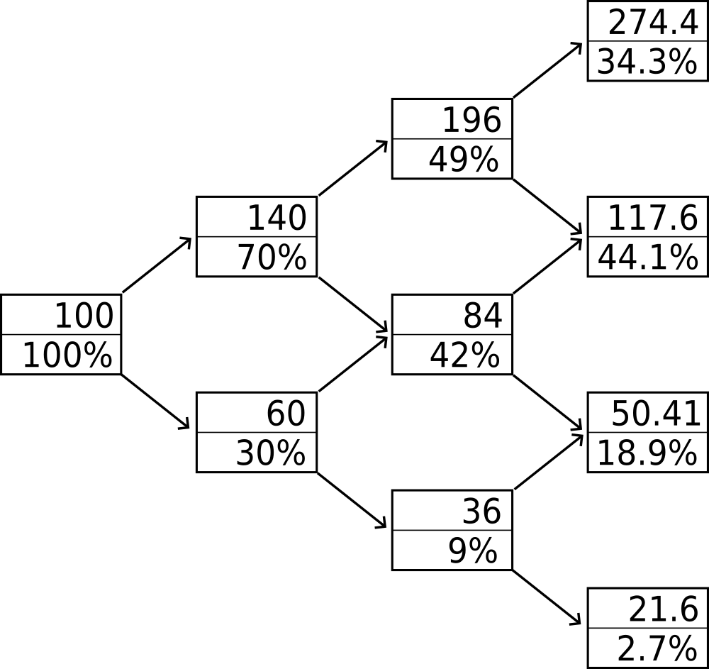
Optimized portfolio in a binomial tree. — Figure 3: Optimized portfolio with 40% fluctuations in a binomial tree.

Summing up, reducing the ±90% risky position to 44.4% of the portfolio increases expected returns in spite of lowering total payoffs. For some better intuition, Figure 3 shows how fluctuations of only 40% benefit investors. While absolute gains drop, they are now more evenly distributed with a total of 78.4% of investors making profits!

Mathematical Foundations

In the section on the correct calculation of returns, it was postulated that the natural logarithm is best suitable to assess investment risk and probability of success. This will now be proven. Afterwards follows a derivation of the formula for the optimization of portfolio returns under idealized conditions.

Why the Natural Logarithm for Calculating Returns?

The natural logarithm measures the speed of exponential growth, which corresponds to the ideal performance of investment portfolios where the reinvestment of regular earnings dominates the accumulation of total value in the long run. For fixed-income investments, the resulting exponential growth in value is known as compound interest effect. As reinvestment periods become shorter, compound interest approaches an exponential function having a base of Euler’s number e^[4]. Assuming short reinvestment periods, as in actively traded brokerage accounts, the growth with long-term rate of return r of a portfolio B over time t (in years) will then be:

B(t) = B(0) \cdot exp(r \cdot t)

The exponential function has the following very useful property:

\begin{aligned} exp(x) \cdot exp(y) = exp(x+y) \end{aligned}

Similarly for the inverse function, the logarithm:

ln(X \cdot Y) = ln(X) + ln(Y)

So exponential function and logarithm complement each other in converting sums to products. For instance, if a portfolio grows in two time steps by factors X and Y, then the values x and y, which can simply be added up in the argument of the exponential function, result from taking logarithms:

\begin{aligned} x := ln(X)\\ y := ln(Y) \end{aligned}

More generally, the performance of a portfolio B can be understood as the product of a long chain of consecutive financial transactions F. With an initial cost of B₀, the portfolio value B_n after n transactions is:

B_n = B_0\prod_{i=1}^{n}F_i

Each factor F_i expresses the return on individual transactions. This return can be specified both in absolute gains and logarithms.

\begin{aligned} F_i &= \frac{B_i}{B_{i-1}} = 1 + G_i\\ F_i &= exp(ln(\frac{B_i}{B_{i-1}})) = exp(f_i) \end{aligned}

Applied to a chain of n transactions, we get:

B_n = B_0~exp(ln(\prod_{i=1}^{n}F_i))

In contrast to the absolute profits G_i, the logarithmic returns f_i truly add up in terms of growth:

B_n = B_0~exp(\sum_{i=1}^{n}f_i)

The portfolio increases in value if and only if the mean of logarithmic returns f_i is above zero:

\begin{aligned} \bar{f} &= \frac{1}{n} \sum_{i=1}^{n}f_i\\ \bar{f} &> 0~~\mathrm{for~gains} \end{aligned}

For portfolio optimization and better risk assessment, it is sufficient to look at the logarithmic returns independently of the time elapsed between individual transactions. However, performance is also easy to measure from a logarithmic point of view. Simply divide the sum of the logarithmic returns f_i by the total time elapsed to obtain the long-term return r:

r = \frac{1}{t} \sum_{i=1}^{n}f_i

Derivation of Optimal Fluctuations

To optimize portfolios, the range of fluctuation for maximum returns can be calculated for a known probability of rising rates. With g as the absolute value of the range of fluctuation and P_u as the probability of positive outcomes, the formula for the return r is:

\begin{aligned} r &= ln(1+g)P_u\\ &~+ ln(1-g)(1-P_u) \end{aligned}

At the point of optimal fluctuation, the first derivative of the rate of return must be zero.

\begin{aligned} \frac{\partial r}{\partial g} = 0 \end{aligned}

With ln(x)’ = 1/x and the chain rule the first derivative is:

\begin{aligned} \frac{\partial r}{\partial g} &= P_u \frac{1}{1+g}\\ &~+ (1-P_u)(-1) \frac{1}{1-g} \end{aligned}

After some transformations we get:

\begin{aligned} g^2 -2P_u~g +2 P_u -1 = 0 \end{aligned}

Quadratic equations have the following general solution formula:

\begin{aligned} &a g^2 + bg + c = 0\\ &g_{1,2} = \frac{-b~\pm \sqrt{b^2 - 4ac}}{2a} \end{aligned}

Plugging in coefficients, the solutions are:

g_{1,2} = P_u~\pm \sqrt{P_u^2 - 2P_u + 1}

The maximum then falls on the smaller of the two solving values:

g = P_u - \sqrt{P_u^2 - 2P_u + 1}

Monte Carlo Simulation of Returns

Significantly more meaningful results than under the simplifying model assumptions of this article can be obtained using a Monte Carlo simulation of returns^[5]. Such an approach also covers relatively improbable scenarios resulting in a total loss and therefore allows for a better assessment of overall risks.

Optimal fluctuation ranges derived in the scope of this article should be taken as upper limits for volatile positions. No one can guarantee profits from risky financial transactions and the author assumes no liability in this regard.